TDM 10100: R Project 1 — 2024
Motivation: The goal of this project is to get you comfortable with the basics of operating in Jupyter notebooks as hosted on Anvil, our computing cluster. If you don’t understand the code you’re running/writing at this point in the course, that’s okay! We are going to go into detail about how everything works in future projects.
Context: You to not need any background to get started in The Data Mine. If you never programmed before, that is totally OK! If you never worked with data before, that is totally OK too! We will spend most of our time learning how to work with data, in a practical way.
Scope: Anvil, Jupyter Labs, Jupyter Notebooks, R, bash
Dataset(s)
This project will use the following dataset(s):
-
/anvil/projects/tdm/data/icecream/breyers/reviews.csv -
/anvil/projects/tdm/data/icecream/bj/products.csv
Questions
Question 1 (2 pts)
First and foremost, welcome to The Data Mine! We hope that throughout your journey with us, you learn a lot, make new friends, and develop skills that will help you with your future career. Throughout your time with The Data Mine, you will have plenty of resources available should you need help. By coming to weekly seminar, posting on the class Piazza page, and joining Dr. Ward and the TA team’s office hours, you can ensure that you always have the support you need to succeed in this course.
The links to Piazza are:
Dr Ward is also available on Monday mornings in the Hillenbrand dining court from 8:30 AM to 11:20 AM. He is also available on Monday afternoons during 4:30 PM to 5:20 PM on Zoom at this URL: purdue-edu.zoom.us/my/mdward/
|
If you did not (yet) set up your 2-factor authentication credentials with Duo, you can set up the credentials here: the-examples-book.com/book/setup If you are still having issues with your ACCESS ID, please send an email containing as much information as possible about your issue to datamine-help@purdue.edu |
Let’s start off by starting up our first Jupyter session on Anvil! We always use the URL ondemand.anvil.rcac.purdue.edu and the ACCESS username that you were assigned (when you setup your account) and the ACCESS password that you chose. These are NOT the same as your Purdue account!
|
These credentials are not the same as your Purdue account. |
In the upper-middle part of your screen, you should see a dropdown button labeled The Data Mine. Click on it, then select Jupyter Notebook from the options that appear. If you followed all the previous steps correctly, you should now be on a screen that looks like this:
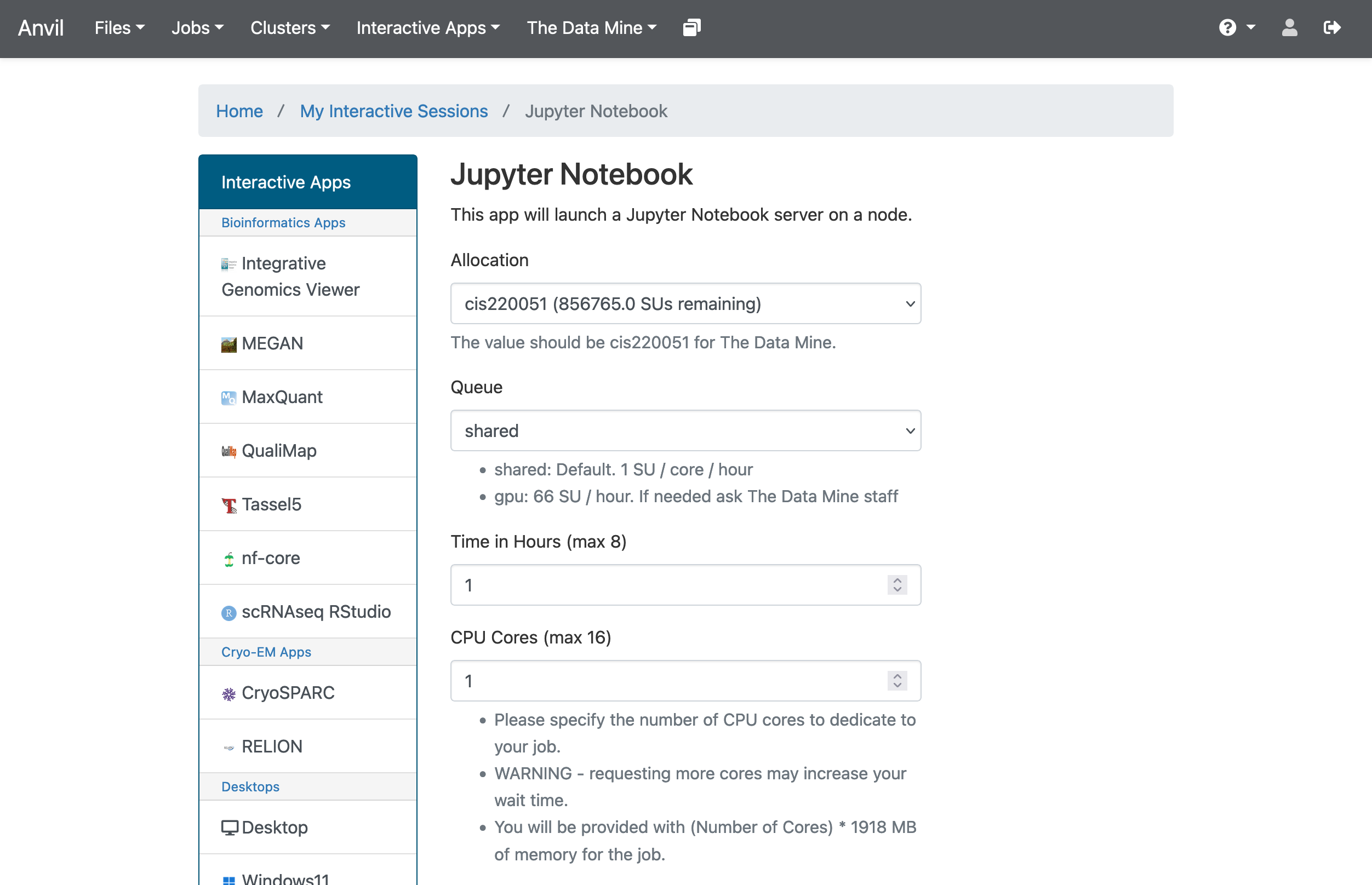
If your screen doesn’t look like this, please try and select the correct dropdown option again or ask one of the TAs during seminar for more assistance.
|
Jupyter Lab and Jupyter Notebook are technically different things, but in the context of seminar we will refer to them interchangeably to represent the tools you’ll be using to work on your projects. |
There are a few key parts of this screen to note:
-
Allocation: this should always be cis220051 for The Data Mine
-
Queue: again, this should stay on the default option
sharedunless otherwise noted. -
Time in Hours: The amount of time your Jupyter session will last. When this runs out, you’ll need to start a new session. It may be tempting to set it to the maximum, but our computing cluster is a shared resource. This means every hour you use is an hour someone else can’t use, so please ONLY reserve it for 1-2 hours at a time.
-
CPU cores: CPU cores do the computation for the programs we run. Just as we mentioned with the hours per session, it may be tempting to request a large number of CPU cores and set it to the maximum, but our computing cluster is a shared resource. This means every computational core that you use is one that someone else can’t use, and we only have a limited number of cores assigned to our team, so please ONLY reserve 1 or 2 cores at a time, unless the project needs more cores. (By the way: All programs require memory to run as well. On Anvil, we will request one or more CPU cores to run our Jupyter Notebooks for Seminar. Each CPU core requested is also allocated 1896MB (1.9GB) of memory. Even if a program requires just a single CPU core for computing it may require, for example, 7GB of memory. This means we must request 4 CPU cores to get sufficient memory (1.9GB times 4 CPU cores gives us 7.6 GB of memory). We have determined in advance the number of CPU cores (and thus memory) will be required for each project and will tell you how many CPU cores you should use.)
|
The Jupyter Lab environment will save your work at regular intervals, so that at the end of a session, your work should be automatically saved. Nonetheless, you can select File from the menu and Save Notebook any time that you want. (It is not necessarily, because the notebooks save automatically, but you can still save anytime if you want to.) |
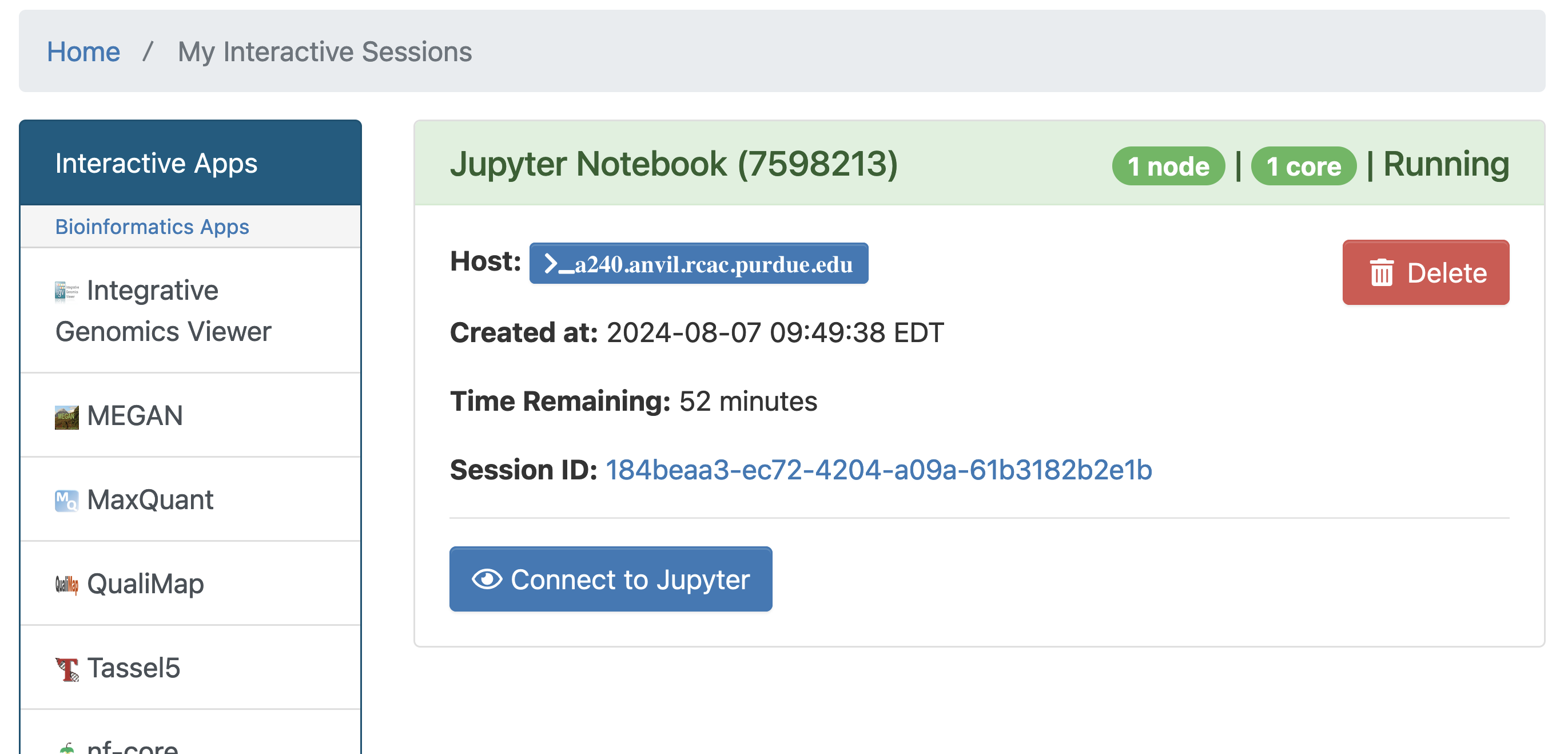
With the key parts of this screen explained, go ahead and select 1 hour of time with 1 CPU cores and click Launch! After a bit of waiting, you should see something like below. Click connect to Jupyter and proceed to the next question!
|
You likely noticed a short wait before your Jupyter session launched. This happens while Anvil finds and allocates space for you to work. The more students are working on Anvil, the longer this will take, so it is our suggesting to start your projects early during the week to avoid any last-minute hiccups causing a missed deadline. |
Download the project template, as described here: the-examples-book.com/projects/templates and then test some of the examples from our helpful page about kernels: the-examples-book.com/projects/kernels
For this first question, from the kernels page above, load the head of the airports data set in Python. (We will focus on R but we will learn some Python later, so it is good to try things from time to time.)
import pandas as pd
myDF = pd.read_csv("/anvil/projects/tdm/data/flights/subset/airports.csv")
myDF.head()
Just try this Python code using the seminar kernel (not the seminar-r kernel) and make sure that you can see the first six rows of the airports data frame.
-
Use Python to show the output with the first six rows of the airports data frame.
Question 2 (2 pts)
As you continue to get comfortable with Jupyter Lab, you might want to read more about Jupyter Lab (this is optional). We want you to get comfortable with switching kernels in Jupyter Lab when needed. The different options that you see (like the seminar kernel and the seminar-r kernel) in the upper right hand of the screen are called kernels (please read the kernel documentation; this is the same as the documentation from Question 1).
When you first open the template, you may get a pop-up asking you to select what kernel you’ll be using. Select the seminar kernel (not the seminar-r kernel). If you do not get this pop-up, you can also select a kernel by clicking on the upper right part of your screen that likely says something similar to No Kernel, and then selecting the kernel you want to use.
Use the seminar kernel with R, and %%R cell magic, to (again) display the first six lines of the airpors data frame, but this time in R:
%%R
myDF <- read.csv("/anvil/projects/tdm/data/flights/subset/airports.csv")
head(myDF)
Now do this again, using the seminar-r kernel with R, and notice that you do NOT need the %%R cell magic with the seminar-r kernel. You can do all of this in the same Jupyter Lab notebook, just by changing the kernel.
myDF <- read.csv("/anvil/projects/tdm/data/flights/subset/airports.csv")
head(myDF)
You have now loaded the first six lines of the airports data frame in three ways (once in Question 1, and now a second and a third time in Question 2).
A Jupyter notebook is made up of cells, which you can edit and then run. There are two types of cells we’ll work in for this class:
-
Markdown cells. These are where your writing, titles, sections, and paragraphs will go. Double clicking a markdown cell puts it in
editmode, and then clicking the play button near the top of the screen runs the cell, which puts it in its formatted form. More on this in a second. For now, just recognize that most markdown looks like regular text with extra characters like#,*, and-to specify bolding, indentation font, size, and more! -
Code cells. These are where you will write and run all your code! Clicking the play button will run the code in that cell, and the programming language is specified by the language or languages known by the kernel that you chose.
For each question in The Data Mine, please always be sure to put some comments after your cells, which describe all of the work that you are doing in the cells, as well as your thinking and insights about the results.
|
Some common Jupyter notebooks shortcuts:
|
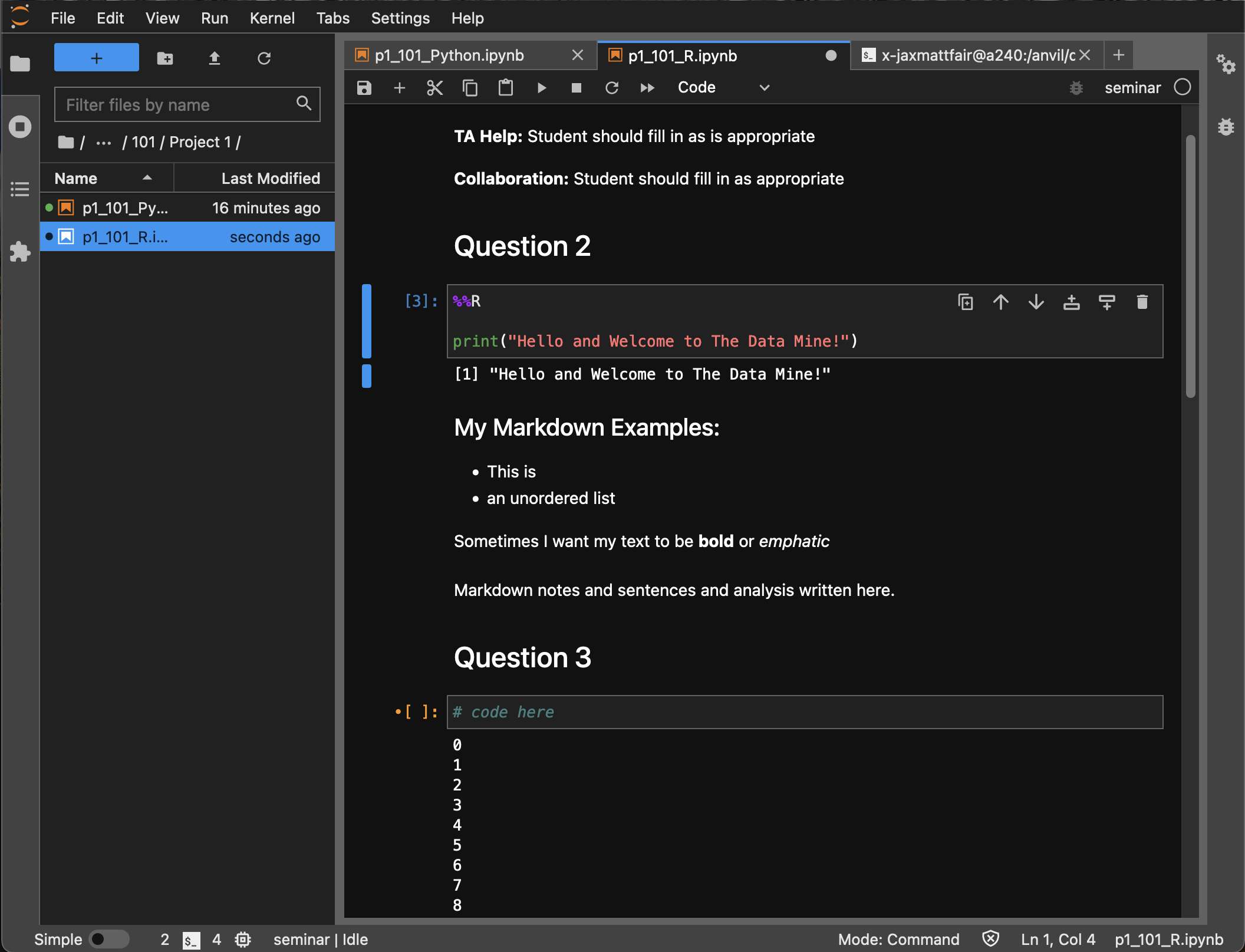
As this is our first real task of the semester, you’ll find a photo below of what your completed Question 2 may look like. Note that yours may differ slightly.
-
Use R to show the output with the first six rows of the airports data frame, and do this two ways: once using R with the
seminarkernel, and once using R with theseminar-rkernel. -
Be sure to document your work from Question 2 (and from Question 1, and indeed from all of the questions throughout your months and years in The Data Mine), using some comments and insights about your work.
Question 3 (2 pts)
In Question 3, copy the following R code into a code cell and run it. This will load the data from an ice cream reviews data set into a data frame, and then will show how much space (in bytes) that your data frame is taking up!:
%%R
myDF <- read.csv("/anvil/projects/tdm/data/icecream/breyers/reviews.csv")
object.size(myDF)
Now let’s do the same thing but in Bash! Create a new code cell below the one you just ran (refer to the hint in the last question for a shortcut on how to do this), and copy in the below code:
%%bash

echo $(du /anvil/projects/tdm/data/icecream/breyers/reviews.csv --bytes | cut -f1) bytes
Running this should give you a smaller output than the R output. This is because in bash, we are checking the size of the stored data, while in Python we are reading the data into a dataframe that has a bit more memory associated with it to make it easier to work with.
|
Notice that |
As a side note, bash is an extremely important foundational tool to working with data and computers more generally. As a 'command line tool', bash is essentially a foundational programming language, and has a lot of fast, efficient, and useful tools that are useful no matter what project you’re working on. From navigating through file directories, to writing basic scripts, to locating and running programs, bash is hiding in the background of most everything your computer does.
Take note of the %%bash line in the cell you just ran. This is called cell magic, and it tells our kernel that we want it to run our code as a different language than the default. As an added example, writing %%python will allow us to run code in the Python programming language.
|
For more information on cell magic and how it works, please refer to this page. |
To further cement your understanding of cell magic, we are going to translate one more bit of code from R to Bash. Let’s take the print() code from the last problem and convert it to its Bash equivalent! As a reminder, here is the R code to translate to Bash
%%R

print("Hello and Welcome to The Data Mine!")|
Printing in Bash can be done using the |
-
The code and results of running the code for each language and task in the question.
-
The Bash equivalent of the
print()statement from the last problem, and the results of running it.
Question 4 (2 pts)
Great work making it this far! At this point, you should now be pretty comfortable running code in Jupyter Notebooks.
In the next 2 questions we are going to introduce some new code that will allow us to read in large datasets and begin to work with them! If you don’t understand the specifics, that’s okay for now. For now, let’s just learn by doing. To start, run the following R code:
%%R

my_df <- read.csv("/anvil/projects/tdm/data/icecream/breyers/reviews.csv")
print(dim(my_df))
head(my_df)
The breakdown of this code is as follows:
-
We use cell magic to make sure the
seminarkernel knows to read our code in the R language -
We use the
read.csvfunction to read the data from the given file into a dataframe we callmy_df. -
We print the dimensions of the dataframe,
my_df. You should see an output of "[1] 5007 8" -
We print the
headof the dataframe, which is just the first 5 rows of our dataframe and the column headers (if they exist).
For the last part of this question, we want you to create a new code cell and write some R to print the names of the columns of our dataframe. If you do everything correctly, you should see the columns are named key, author, date, stars, title, helpful_yes, helpful_no, and text. If you’re struggling, take a look at the hint below:
|
R has two built-in functions, called |
-
The result of runnning the provided code that reads in a dataframe and prints its shape.
-
A code cell that prints the names of the columns in
my_df
Question 5 (2 pts)
Let’s take a second to reflect on everything you did and learned during this project. First, you learned how to Launch a Jupyter Notebook session on the Anvil supercomputing cluster. Next you learned about uploading files to Anvil, the general structure of Jupyter notebooks, and how to manipulate the contents of a notebook to fit your working style. Finally, you learned how to write and run some basic code in Jupyter notebooks, including how to read in data!
In this last question, we are going to try and put everything you learned today together. In the previous question, you read a file on Breyer’s ice cream reviews into a dataframe called my_df and printed the number of columns and rows in the dataframe. Finally, we had you write some code to print the names of the columns of my_df
In this question, we want you to read a file on Breyers’s ice cream products into a dataframe called BreyProd_df. The path to the file is /anvil/projects/tdm/data/icecream/bj/products.csv. Next, print the number of rows and columns in BreyProd_df, and then print the names of the columns in BreyProd_df.
|
The code needed to solve this problem is almost identical to that of the last problem. If you’re struggling, considering revisiting Question 4 and trying to better understand what is going on in that code, and feel free to copy the code from Question 4 into Question 5 and modify it directly. |
One way you can validate that your code is working correctly is comparing the results of your code that outputs the number of rows/columns in the dataframe with the code that outputs the names of the columns in the dataframes. The number of columns in the dataframe should match the number of names printed.
Finally, make sure that your name is at the top of the project template. If you used outside resources (like Stack Overflow) or got help from TAs, make sure to note where you got assistance from, and on what part of the project they assisted you, in the appropriate sections at the top of the template.
-
Code that reads the
products.csvfile into a dataframe -
Code that prints the shape of the resulting dataframe
-
Code that prints the names of the columns in the resulting dataframe
Submitting your Work
Congratulations! Assuming you’ve completed all the above questions, you’ve just finished your first project for TDM 10100! If you have any questions or issues regarding this project, please feel free to ask in seminar, over Piazza, or during office hours. Prior to submitting, make sure you’ve run all of the code in your Jupyter notebook and the results of running that code is visible. More detailed instructions on how to ensure that your submission is formatted correctly can be found here. To download your completed project, you can right-click on the file in the file explorer and click 'download'.
Once you upload your submission to Gradescope, make sure that everything appears as you would expect to ensure that you don’t lose any points. At the bottom of each 101 project, you will find a comprehensive list of all the files that need to be submitted for that project. We hope your first project with us went well, and we look forward to continuing to learn with you on future projects!!
-
firstname_lastname_project1.ipynb
|
You must double check your You will not receive full credit if your |